Speed up PostgreSQL® pgvector queries with indexes

Using AI, it’s possible to find similar text information, photos or products in a database. As the number of searches increases, performance can be a problem, though.In this article, I’ll show you how PostgreSQL® indexes can help.

We’re going to use PostgreSQL’s pgvector extension. It enables you to store AI embeddings, which are representations of information, and enables you to perform similarity searches on them. Pgvector has a couple of features that make it particularly popular. It supports hybrid searches, mixing standard and vector queries. For example, someone shopping online might want to search for shoes that look like a photo of their existing pair (a vector search), and that cost less than $100 (a standard database query). Pgvector also enables retrieval-augmented generation (RAG), where information from the database gives additional context to generative AI, improving the quality of the output and reducing hallucinations.

This tutorial explains:

• The basics of vector similarity
• How pgvector can be used for vector similarity searches
• How indexes of various types can help to speed up searches
• The possible tradeoffs in output quality when using indexes

See our previous blog for a refresher on what embeddings are and how pgvector can be used for face recognition.

To get insights about your database performance and improvement suggestions, check out EverSQL by Aiven

Understanding vector queries

In the AI world, embeddings are a representation of a piece of information (such as text, image, sound, or video). They are expressed as an array of numbers.

AI models such as OpenAI’s text-embedding-ada-002can generate embeddings from text (see the image below). These embeddings are always the same length, no matter how long the source text is. In the case of ada-002, the embeddings are 1536 elements long. The embeddings can be compared to find text with a similar meaning.

But how does this embedding comparison work? We can picture the embeddings as points in an N-dimensional space. In the case of text-embedding-ada-002, it would be a 1536-dimension space.

To find information similar to a particular search query, the AI model would:

1. Create an embedding for the search query, using the same method used for the stored data. Information with a similar meaning should be represented by embeddings with similar values. These embeddings would be closer to each other in the N-dimensional space.
2. Search the N-dimensional space to find the embeddings that are closest to the search query.

It's hard to imagine a 1536 dimension space, so to keep things simple, we’ll visualize the data in a two-dimensional space. In the image below, you can see the search query embedding in yellow in the center, and the six closest results we’d want to find in red.

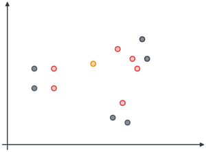
In that image, we’re plotting the data as coordinates. However, the embeddings can be considered as vectors. These are mathematical objects that have a length and direction. They’re represented by an arrow that starts at the graph’s origin at [0,0] in the bottom left and extends to the vector position. You’ll see these shortly.

There are several ways that the similarity of vectors can be measured. Let’s create a PostgreSQL environment where we can explore the different approaches using pgvector.

Setting up a PostgreSQL playground

We’re going to spin up an Aiven for PostgreSQL database. Follow these steps:

1. Access the Aiven Console.
2. Select Create service.
3. Select Aiven for PostgreSQL.
4. Select the cloud provider and region.
5. Select the plan (the hobbyist or even the free plan would be enough).
6. Provide the service a name, such as pg-pgvector-index-test.
7. Click on Create service.
8. Connect to PostgreSQL. To do this, wait until the service is in the RUNNING state, grab the Service URI and, with psql already installed locally, connect to PostgreSQL with:

    psql <SERVICE_URI>
   

9. Create the pgvector extension using CREATE EXTENSION vector;
10. Add some data using the following code:

    CREATE TABLE VECTOR_TEST (id int, name text, vctr vector(2));
    
    INSERT INTO VECTOR_TEST VALUES
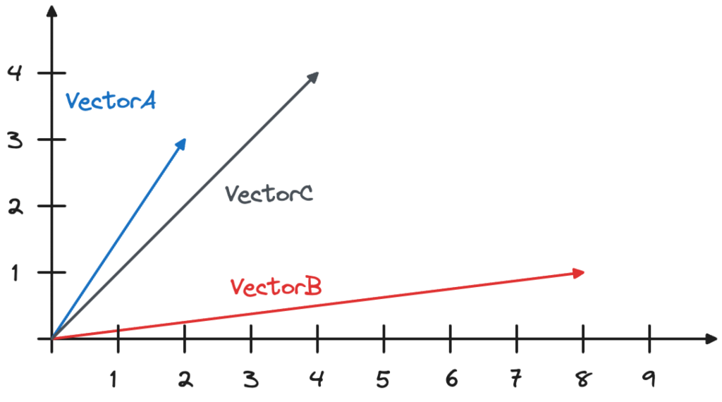
        (1, 'VectorA', '[2,3]'),
        (2, 'VectorB', '[8,1]');
    

We now want to calculate the similarity between the two vectors (VectorA and VectorB) and a third vector (VectorC) with coordinates [4,4], as shown in the image below.

Understanding how similarity metrics work

Similarity metrics define the distance between two embeddings (or vectors). There are a lot of different similarity metrics we could use, but we’ll define the three basic ones: distance, inner product and cosine.

Distance

The distance similarity metric calculates the Euclidean distance between two vectors using the formula $\sqrt{Δx^2+Δy^2}$, as shown in the image below. You can visualize this by drawing a right-angled triangle, with the long side connecting the vectors. To calculate the length of the line connecting the vectors length, use Pythagoras’ theorem.

Embeddings with a lower distance metric are closer together in the space, and so represent content with a more similar meaning.

The distance similarity is measured using PostgreSQL <-> operator.

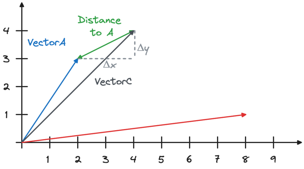
The similarity between VectorA and VectorC is calculated as $\sqrt{(4-2)^2+(4-3)^2}$ which equals 2.23606797749979. The similarity between VectorB and VectorC will be $\sqrt{(8-4)^2+(4-1)^2}$, which equals 5.

Let’s run the following query:

SELECT name, 
vctr <-> '[4,4]' distance 
from VECTOR_TEST;

The result is what we expected:

name     |     distance
---------+------------------
VectorA   | 2.23606797749979
VectorB   |                5

(2 rows)

The Euclidean distance is ideal for finding similar vectors if all the components of a vector have equal importance, and if they are normalized so the numbers are on the same scale (for example, between 0 and 1).

Cosine

We said that the distance metric is ideal for normalized data, but what if there could be large differences in the scale of the data?

The cosine similarity calculates the difference in the angle between the two vectors, measuring how closely the two vectors are pointing in the same direction. The cosine similarity metric does not otherwise consider the vectors’ positions in the space. The vector positions could be a long way apart.

For example, imagine a certain element contains the “number of times Pizza is mentioned in the document”, with the length of the line representing the frequency and the position of the vector representing the idea of pizza. You could use the cosine distance to find other documents containing the idea of Pizza, rather than focusing on documents that mention Pizza a certain number of times. By contrast, a distance search on this element might be more likely to find items with a similar frequency, than items with a similar idea.

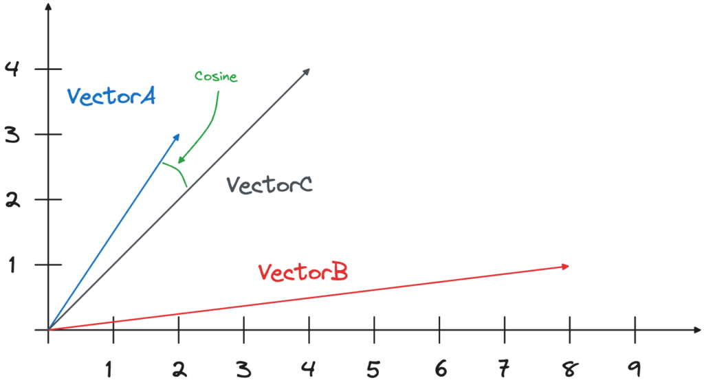
In the case of VectorA and VectorC the cosine difference is calculated as $((Xa*Xc)+(Ya*Yc))/(\sqrt{Xa^2+Ya^2)}*\sqrt{Xc^2+Yc^2)})$, with the result being 0.9805806756909202.

The distance similarity is measured using <=>.

Let’s try it:

SELECT name, 
1 - (vctr <=> '[4,4]') cosine_similarity 
from VECTOR_TEST;

The result is in line with the above calculation. The angle between VectorAand VectorC is way smaller than the one between VectorB and VectorC, therefore the cosine similarity of the VectorA is greater. In the output, a higher number represents greater similarity.

name   | cosine_similarity
---------+--------------------
VectorA | 0.9805806756909202
VectorB | 0.7893522173763263

(2 rows)

Inner product

The inner product allows you to measure both the space between vectors and how well aligned they are. Although the inner product works well where the elements of a vector are normalized and have equal importance, it also works where not all the elements have an equal weight.

To see how it’s useful, imagine you have an AI model that creates elements expressing how often a certain word appears in a document. The word Margherita would appear often in articles about pizza and about queens of Italy. These are two totally different contexts, of course. Using the inner product, you can get a sense of whether a query and a result have a similar direction, which will reflect how close their meanings are. You can also get a sense of scale: how many mentions there are of the word.

The inner product calculates the area of the parallelogram created when you join the vectors as shown in the image below.

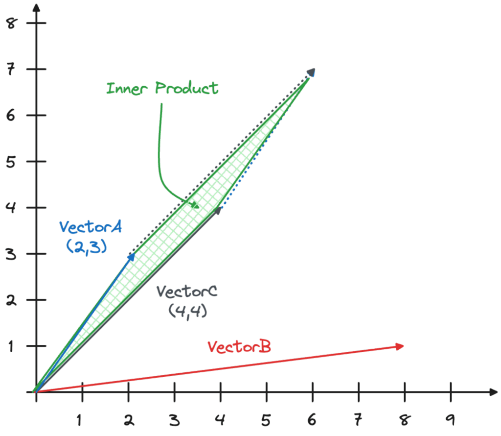
The calculation is made by multiplying each of the coordinates and then summing the result with the formula $(Xa*Xc)+(Ya*Yc)$. This is known as the dot product. The result, in the case of VectorA and VectorC, is (2*4)+(3*4)=20.

The inner product is measured using <#>.

Try executing the query against the PostgreSQL database with this code:

SELECT name, 
(vctr <#> '[4,4]') * -1 inner_product 
from VECTOR_TEST;

We multiply the result by -1 because PostgreSQL returns the negative inner product and we want to make the result positive. The result is in line with the formula:

name   | inner_product
---------+---------------
VectorA |            20
VectorB |            36

(2 rows)

Testing the vector similarity theory at scale

As we have just seen, each coordinate needs to be evaluated to calculate the vector similarity.. If our data set has N rows containing vectors with M dimensions, we’ll need to perform at least N*M calculations to measure the similarity.

If we are working with long vectors, such as the ones coming from AI embeddings (usually in the range of 1000 elements), we would need to perform at least 1000 calculations for every row in our data set to calculate full vector similarity. This would not scale well, but there are several optimizations that can help.

To experiment, let’s download the OpenAI pre-computed Wikipedia article embeddings, which are available in the OpenAI Cookbook. The file contains embeddings for 25,000 Wikipedia articles.

Follow these steps:

1. Open the terminal.
2. Download the zip file:

    wget https://cdn.openai.com/API/examples/data/vector_database_wikipedia_articles_embedded.zip
   

3. Unzip it with:

    unzip vector_database_wikipedia_articles_embedded.zip -d .
   

4. Connect to PostgreSQL:

    psql <SERVICE_URI>
   

5. Create a table named articles:

    CREATE TABLE IF NOT EXISTS articles (
        id INTEGER NOT NULL,
        url TEXT,
        title TEXT,
        content TEXT,
        title_vector vector(1536),
        content_vector vector(1536),
        vector_id INTEGER
    );
   

6. Load the table with 25,000 articles and related embeddings:

    \COPY public.articles (id, url, title, content, title_vector, content_vector, vector_id) FROM 'vector_database_wikipedia_articles_embedded.csv' WITH (FORMAT CSV, HEADER true, DELIMITER ',');
   

Now, if we want to retrieve the top 10 articles which have a similar meaning to Pineapple Pizza we can issue the following query using the distance similarity:

with data as (
    select '[0.02338707074522972, -0.017537152394652367, 0.014360039494931698, -0.025202563032507896, -0.017234569415450096, 0.0018643466755747795, -0.013893559575080872, -0.009581765159964561, 0.006732450798153877, -0.03714194521307945, 0.021848944947123528, 0.008800094947218895, -0.012323915027081966, 0.005071401130408049, -0.0010046670213341713, 0.008768576197326183, 0.03086336888372898, -0.010867739096283913, -0.001483755186200142, -0.006631589960306883, 0.00044835725566372275, -0.01773887313902378, 0.01492738164961338, -0.01236173789948225, 0.022340642288327217, 0.009815005585551262, 0.008579461835324764, -0.00020428228890523314, 0.011605282314121723, 0.014309609308838844, 0.05285099893808365, -0.0039430223405361176, -0.012985813431441784, -0.01689416542649269, -0.02065122500061989, 0.0007375437417067587, -0.003873680718243122, -0.010886650532484055, 0.001689416472800076, -0.022769300267100334, 0.01762540452182293, -0.03451956808567047, -0.009644802659749985, -0.023160135373473167, -0.042336273938417435, 0.0012576066656038165, -0.002456903224810958, -0.01002933457493782, -0.0002019183593802154, -0.01362880039960146, 0.018482720479369164, 0.009733055718243122, -0.028140131384134293, -0.005036730319261551, 0.005433869548141956, 0.010357131250202656, -0.0082012340426445, -0.023424893617630005, -0.00740065285935998, -0.01778930239379406, 0.01135313045233488, 0.0030967381317168474, -0.03149374946951866, 0.003227541921660304, -0.0014018059009686112, 0.005799489561468363, 0.003656199900433421, -0.011605282314121723, 0.021647224202752113, -0.008012120611965656, 0.021382465958595276, 0.007583462633192539, 0.01825578324496746, -0.02455957606434822, 0.013111889362335205, 0.006612678524106741, -0.01002933457493782, -0.013843129388988018, 0.0011441383976489305, 0.009436777792870998, 0.026501145213842392, -0.012424775399267673, 0.0019179289229214191, 0.038327060639858246, 0.017511935904622078, 0.0007111466256901622, -0.0398399718105793, 0.014902166090905666, 0.01705806329846382, -0.0058120968751609325, -0.01645289920270443, 0.005802641157060862, -0.0021842641290277243, 0.013200142420828342, -0.038629643619060516, 0.012626497074961662, -0.011674623936414719, 0.025063879787921906, 0.004006060305982828, -0.02570686675608158, -0.0014152014628052711, 0.01905006170272827, -0.014082673005759716, -0.02687937207520008, 0.002307188231498003, -0.007684323471039534, -0.0012316035572439432, -0.023550970479846, 0.023122312501072884, 0.0026712322141975164, -0.011838522739708424, 0.03119116649031639, 0.010023030452430248, -0.022907983511686325, 0.002924959873780608, 0.004500907845795155, 0.015116495080292225, 0.007148500997573137, -0.024143526330590248, -0.04362224414944649, 0.028316637501120567, 0.0036971743684262037, 0.027333244681358337, -0.00706024793908, 0.02720716968178749, 0.0025388526264578104, 0.001517638098448515, -0.021458109840750694, 0.004188870079815388, -0.0099032586440444, 0.027434106916189194, 0.00335992150940001, 0.013729660771787167, -0.005878286901861429, -0.0066757164895534515, 0.005052489694207907, -0.011208144016563892, -0.017511935904622078, -0.02303405851125717, -0.04329444840550423, 0.016087278723716736, 0.03217455744743347, -0.020260389894247055, 0.02179851569235325, -0.02310970425605774, 0.01286604069173336, 0.014196141622960567, 0.008674019016325474, -0.007785184308886528, -0.018268391489982605, 0.02343750186264515, 0.00034887553192675114, 0.0004243240400683135, 0.009991511702537537, 0.014435685239732265, 0.0001373044797219336, -0.028417497873306274, 0.011056852526962757, 0.005695476662367582, -0.009323309175670147, 0.010016726329922676, -0.016490722075104713, -0.010924472473561764, -0.008692930452525616, 0.012815610505640507, 0.03946174308657646, 0.004904350731521845, 0.023513147607445717, -0.0021291060838848352, -0.005043034441769123, -0.0021763844415545464, 0.04074771702289581, -0.042714498937129974, 0.025719475001096725, -0.007028728723526001, 0.007659108377993107, -0.018596189096570015, -0.003369377227500081, 0.01211589016020298, 0.011662016622722149, -0.005188021343201399, -0.00453557912260294, 0.013414471410214901, 0.032729290425777435, -0.01222305465489626, -0.03595683351159096, -0.00804994348436594, -0.027333244681358337, -0.007898651994764805, -0.005610375665128231, 0.013326218351721764, 0.028467928990721703, 0.01912570744752884, 0.0004979996010661125, -0.6854491829872131, -0.014700444415211678, 0.01694459468126297, -0.04112594574689865, 0.022857552394270897, 0.042058903723955154, 0.005216388497501612, -0.010672321543097496, -0.0071232859045267105, -0.022605400532484055, -0.003879984375089407, 0.017776696011424065, 0.038377489894628525, -0.0006792336935177445, -0.02174808457493782, -0.023160135373473167, 0.018217960372567177, -0.013225357048213482, -0.016162924468517303, 0.020840339362621307, -0.0008691354305483401, 0.0037728198803961277, 0.01689416542649269, 0.00024269602727144957, 0.040016476064920425, 0.0029958775267004967, 0.018570972606539726, -0.015683837234973907, -0.004273971542716026, 0.013691837899386883, -0.02469825930893421, 0.008888348005712032, 0.005310945212841034, -0.00878748670220375, 0.047707103192806244, 0.009272878989577293, -0.03192240744829178, 0.01286604069173336, 0.00370032642967999, 0.03729323670268059, -0.010212143883109093, -0.018709657713770866, 0.02627420797944069, 0.0015113343251869082, -0.024710867553949356, -0.00931700598448515, 0.016818519681692123, -0.0068270075134932995, 0.014813913032412529, -0.007778880186378956, 0.02179851569235325, 0.0021338339429348707, 0.0198065172880888, 0.021861553192138672, 0.0033473139628767967, -0.00144593243021518, 0.03991561755537987, 0.00053385243518278, -0.0048034898936748505, -0.008409259840846062, -0.0037034782581031322, 0.008276879787445068, -0.021508540958166122, -0.014977811835706234, -0.012191534973680973, 0.006051640957593918, 0.0014049578458070755, 0.009726752527058125, 0.019655225798487663, -0.010899257846176624, 0.008610980585217476, -0.002247302094474435, -0.014070065692067146, 0.0035742504987865686, 0.024433501064777374, 0.02594641037285328, 0.010218448005616665, 0.00415419926866889, -0.003927262965589762, 0.0017067518783733249, 0.0069593871012330055, 0.00037054481799714267, -0.013994419947266579, 0.0002880045212805271, 0.024622615426778793, -0.002004606183618307, -0.04543773829936981, 0.006168261170387268, 0.012040244415402412, -0.00014479024684987962, 0.027156738564372063, 0.0073943487368524075, -0.012639104388654232, 0.01853315159678459, 0.0016626253491267562, -0.007734753657132387, -0.02927481383085251, 0.012260876595973969, 0.015028242021799088, -0.016440290957689285, -0.02013431489467621, 0.01820535399019718, 0.02362661622464657, -0.012771484442055225, 0.006921564694494009, -0.0072430577129125595, -0.002504181582480669, 0.006161957513540983, 0.04493343457579613, -0.02594641037285328, 0.013401863165199757, -0.02819056063890457, -0.026425499469041824, -0.012292396277189255, 0.018999630585312843, -0.02619856223464012, 0.03126681223511696, -0.025000842288136482, -0.015709051862359047, -0.014574368484318256, -0.0008234329288825393, -0.002515213331207633, 0.015608190558850765, -0.0013332521775737405, -0.008604677394032478, 0.024004843086004257, -0.0018249480053782463, -0.006120982579886913, 0.007823007181286812, -0.001020426512695849, 0.005298337899148464, 0.013263179920613766, 0.0029454471077769995, 0.0029202320147305727, -0.015166925266385078, -0.010691232979297638, 0.013918774202466011, -0.022554971277713776, 0.023311425000429153, -0.034040480852127075, -0.005616679321974516, -0.00044875123421661556, -0.02387876622378826, 0.022164136171340942, -0.0071106781251728535, -0.02010909840464592, -0.00795538630336523, -0.013502724468708038, 0.006795488763600588, 0.009896954521536827, 0.0005756150931119919, -0.030989445745944977, 0.00514389481395483, 0.007457386702299118, 0.017348038032650948, -0.01309928111732006, 0.02310970425605774, 0.001585403922945261, 0.0009061702294275165, -0.035326454788446426, 0.015595583245158195, 0.025845550000667572, 0.002037700964137912, -0.0032968835439532995, 0.007917563430964947, -0.01378009095788002, -0.007961690425872803, -0.0039051997009664774, 0.028392283245921135, -0.016062064096331596, 0.020777301862835884, -0.009959992952644825, 0.003832706017419696, -0.009241360239684582, -0.025895981118083, 0.024168740957975388, -0.00444102194160223, -0.0026428650598973036, 0.0011709295213222504, 0.010552548803389072, -0.012910167686641216, 0.03020777553319931, -0.006997209973633289, 0.02294580638408661, -0.004812945611774921, -0.005897198338061571, 0.003930415026843548, 0.03262843191623688, -0.020537756383419037, 0.0030321243684738874, -0.004217237234115601, 0.02371486835181713, 0.008667714893817902, 0.014082673005759716, 0.019087884575128555, -0.004018668085336685, 0.00436537666246295, -0.008005816489458084, -0.012405863963067532, 0.01907527633011341, -0.0022599096409976482, -0.005266818683594465, 0.010262575000524521, -0.012626497074961662, 0.03641070798039436, -0.02695501782000065, -0.0024364159908145666, -0.027156738564372063, 0.034998659044504166, 0.019667834043502808, 0.001085040275938809, -0.029804332181811333, -0.020260389894247055, 0.0007206022855825722, -0.007533032447099686, 0.04112594574689865, -0.017562367022037506, 0.021533755585551262, 0.005030426662415266, 0.009090068750083447, 0.0038673768285661936, 0.006789184641093016, -0.009840220212936401, -0.0020471566822379827, -0.007848221808671951, 0.013036243617534637, 0.005339312367141247, 0.00012617434549611062, 0.02406788058578968, -0.04286579042673111, -0.0002070401969831437, 0.0191004928201437, -0.005635590758174658, 0.0044000474736094475, 0.027408890426158905, 0.008566854521632195, 0.00746369082480669, 0.0031786875333637, 0.008138196542859077, 0.015809912234544754, 0.005487451795488596, 0.023891374468803406, 0.0061052232049405575, 0.0012631224235519767, 0.008409259840846062, -0.005440173204988241, 0.03754539042711258, -0.012071763165295124, -0.023185350000858307, 0.03827663138508797, -0.008497512899339199, -0.011888952925801277, -0.023677045479416847, 0.027988839894533157, 0.04120158776640892, -0.021306820213794708, -0.005118679720908403, 0.008705537766218185, 0.019340036436915398, 0.02229021117091179, 0.012847129255533218, -0.004062794614583254, -0.0021306818816810846, -0.002497877925634384, -0.0023576184175908566, -0.02196241356432438, 0.00955024641007185, -0.02046211063861847, -0.015103887766599655, -0.0018202201463282108, 0.0006485026679001749, -0.03588118776679039, 0.015860343351960182, -0.020752085372805595, -0.014574368484318256, -0.015444292686879635, -0.0008415563497692347, 0.019680440425872803, 0.0015349735040217638, -0.008522727526724339, -0.010331916622817516, -0.04120158776640892, 0.033737897872924805, 0.003596313763409853, -0.010602978989481926, -0.013137103989720345, -0.014776090160012245, 0.005673413630574942, -0.008087766356766224, 0.005531578324735165, 0.009972600266337395, 0.013590977527201176, 0.019037453457713127, 0.01806667074561119, -0.022189350798726082, 0.0008131892536766827, 0.01823056861758232, -0.007205235306173563, 0.015242571011185646, -0.0013844704953953624, 0.003274820279330015, 0.003823250299319625, -0.013326218351721764, -0.008560550399124622, 0.04682457447052002, 0.0071232859045267105, -0.01143508031964302, -0.004926414228975773, 0.011233358643949032, 0.000963692320510745, 0.010117587633430958, -0.009978904388844967, -0.01675548031926155, -0.015192140825092793, -0.0024253842420876026, -0.005890894215553999, -0.003218086203560233, -0.014385255053639412, 0.026778511703014374, -0.006864830385893583, -0.0006410169298760593, -0.013855736702680588, -0.028089700266718864, 0.01028778962790966, 0.09274140000343323, 0.01647811383008957, 0.011365738697350025, 0.001995150465518236, -0.004157351329922676, 0.0016452899435535073, -0.017663227394223213, -0.008018424734473228, -0.0039430223405361176, -0.027106309309601784, 0.012059155851602554, 0.02090337686240673, 0.00654964055866003, 0.004680566024035215, 0.005950780585408211, -0.009770878590643406, -0.011340523138642311, -0.016906771808862686, 0.00946829654276371, -0.008995512500405312, -0.008781183511018753, 0.00839034840464592, 0.01062819454818964, 0.019440896809101105, 0.019503934308886528, -0.002902896609157324, 0.04715237021446228, 0.03149374946951866, -0.005566249135881662, -0.015973810106515884, -0.020197352394461632, -0.0015909196808934212, 0.0016484417719766498, -0.012065459042787552, 0.0038011870346963406, -0.009480904787778854, 0.019415682181715965, -0.0027279662899672985, 0.027333244681358337, 0.0013545274268835783, -0.00019157619681209326, 0.010199536569416523, -0.003378832945600152, -0.013981812633574009, 0.006921564694494009, 0.004340161103755236, -0.011781788431107998, 0.018860947340726852, -0.010155410505831242, 0.004589161369949579, 0.031998053193092346, 0.0031077698804438114, 0.005755363032221794, -0.005966539960354567, 0.00803733617067337, 0.0011843250831589103, 0.01048951130360365, -0.014902166090905666, 0.018104493618011475, -0.017259784042835236, -0.008239056915044785, -0.013174926862120628, -0.01683112606406212, 0.00045269110705703497, 0.00195417576469481, -0.03116595186293125, 0.0032243900932371616, -0.005928717087954283, -0.013754875399172306, -0.01691938005387783, -0.013326218351721764, -0.013111889362335205, -0.013729660771787167, -0.010325612500309944, 0.01970565691590309, 0.024080488830804825, 0.003873680718243122, 0.0020361251663416624, 0.01970565691590309, 0.018154922872781754, 0.007507817354053259, -0.0129479905590415, -0.01237434521317482, -0.01656636781990528, -0.009739359840750694, 0.027156738564372063, 0.032351065427064896, -0.007753665093332529, 0.015570368617773056, -0.0028634979389607906, 0.02371486835181713, 0.00654964055866003, 0.011327915824949741, 0.00501466728746891, -0.027156738564372063, -0.0070917666889727116, 0.0007670928025618196, 0.007614981848746538, -0.012550851330161095, 0.007211538963019848, -0.010949688032269478, -0.011561156250536442, 0.0058089448139071465, -0.014675229787826538, -0.004305490292608738, 0.0009573885472491384, 0.0029076244682073593, 0.009090068750083447, -0.014334824867546558, -0.007413260173052549, 0.0062502105720341206, 0.0037349972408264875, 0.008024727925658226, 0.016604190692305565, 0.003798035206273198, 0.04387439787387848, -0.021622009575366974, 0.007867133244872093, -0.026450714096426964, -0.01715892367064953, 0.018671834841370583, -0.02128160372376442, -0.0029832699801772833, -0.0023276754654943943, 0.0003541943442542106, -0.02453436143696308, -0.01724717766046524, -0.027736688032746315, -0.014233964495360851, -0.01615031622350216, 0.0002905654546339065, 0.019138315692543983, 9.155274165095761e-05, -0.006294337101280689, -0.008333614096045494, -0.004188870079815388, 0.0005752210854552686, -0.006915260571986437, -0.004920110106468201, -0.031065091490745544, -0.021861553192138672, 0.01331361010670662, -0.00034296573721803725, 0.01945350505411625, -0.020209958776831627, -0.02990519255399704, -0.01853315159678459, -0.009291790425777435, -0.008510120213031769, 0.015646014362573624, 0.007551943883299828, -0.008629892021417618, -0.0004408715176396072, -0.010974903590977192, -0.026173347607254982, -0.020033452659845352, -0.02090337686240673, -0.01905006170272827, -0.005433869548141956, 0.015683837234973907, 0.015393861569464207, 0.01028778962790966, -0.004800338298082352, 0.00028248870512470603, -0.0145869767293334, 0.0018265239195898175, -0.0013427078956738114, -0.0018533150432631373, -0.029653040692210197, 0.027459321543574333, 0.03383876010775566, 0.013338825665414333, 0.0034954531583935022, 0.016352038830518723, -0.012557155452668667, 0.008453385904431343, -0.0003792125207837671, -0.02575729787349701, -0.006833311170339584, -0.01656636781990528, -0.02305927313864231, -0.0029848457779735327, -0.01509127952158451, -0.007898651994764805, 0.02125638909637928, 0.010205840691924095, 0.01495259627699852, 0.0012442111037671566, 0.002913928125053644, -0.006130438297986984, 0.018457505851984024, -0.02950175106525421, 0.006174564827233553, -0.014007027260959148, 0.015759481117129326, -0.0087307533249259, -0.023815728724002838, 0.013414471410214901, -0.02444610930979252, 0.0038957439828664064, 0.010773181915283203, 0.015028242021799088, -0.02387876622378826, -0.014776090160012245, -0.01064080186188221, 0.032401494681835175, -0.0011134074302390218, 0.00971414428204298, 0.005925565026700497, -0.0356290377676487, -0.022933198139071465, -0.01280930731445551, -0.013200142420828342, -0.040066905319690704, 0.014813913032412529, -0.01928960531949997, -0.018659226596355438, 0.017499329522252083, -0.0031172255985438824, -0.030737293884158134, -0.0001579888048581779, 0.01413310319185257, 0.023992234840989113, 0.01328839547932148, 0.02861921861767769, 0.03641070798039436, -0.004708933178335428, -0.013477508910000324, 0.026980232447385788, -0.01893659308552742, -0.02032342739403248, 0.023500539362430573, -0.013036243617534637, 0.011384650133550167, -0.013654015026986599, -0.011933079920709133, 0.02078990824520588, -0.011756573803722858, -0.006120982579886913, 0.017398467287421227, 0.005928717087954283, 0.003331554587930441, -0.021218566223978996, -0.008257968351244926, -0.01678069680929184, 0.012172623537480831, -0.030359065160155296, -0.011933079920709133, -0.001746150548569858, -0.009045942686498165, -0.03222499042749405, 0.013137103989720345, -0.02526560053229332, 0.022819729521870613, -0.007425867952406406, -0.008239056915044785, 0.007142197340726852, -0.009342220611870289, -0.017032848671078682, 0.011132498271763325, 0.0024033209774643183, 0.03194762021303177, -0.005790033843368292, 0.0291739534586668, -0.008138196542859077, 0.006073704455047846, 0.01877269521355629, 0.03310751914978027, 0.00874336063861847, 0.021168136969208717, -0.013679230585694313, -0.0014632679522037506, -0.001120499218814075, -0.00746369082480669, 0.021243780851364136, 0.0025782512966543436, -0.014435685239732265, -0.007886044681072235, -0.014776090160012245, -0.010558852925896645, 0.012134800665080547, 0.010729054920375347, -0.01778930239379406, -0.004705781117081642, -0.010224752128124237, -0.008579461835324764, -0.03850356489419937, 0.003077826928347349, -0.024156134575605392, -0.0065307291224598885, -0.024622615426778793, 0.004718388896435499, 0.015923380851745605, 0.012500421144068241, 0.027408890426158905, 0.016036849468946457, -0.02160940133035183, -0.013162319548428059, -0.015356039628386497, 0.0202729981392622, 0.007066551595926285, 0.0026633525267243385, -0.01642768457531929, -0.0038011870346963406, 0.0025940106716006994, -0.010281486436724663, 0.01562079880386591, -0.02884615585207939, 0.011025333777070045, -0.011075763963162899, 0.005219540558755398, 0.013515331782400608, -0.006083160173147917, 0.0033819847740232944, 0.02179851569235325, 0.0068270075134932995, 0.015709051862359047, -0.002231542719528079, -0.011983510106801987, 0.005881438497453928, -0.009146803058683872, 0.0025498841423541307, 0.0036309845745563507, 0.018482720479369164, -0.016339430585503578, -0.012393256649374962, -0.0010621891124173999, 0.005188021343201399, -0.01427178643643856, 0.010798397473990917, -0.024143526330590248, 0.04914436861872673, -0.008560550399124622, 0.0030132129322737455, -0.007173716090619564, -0.006373134441673756, 0.010905561037361622, 0.024004843086004257, -0.006732450798153877, -0.0077032349072396755, 0.00631640013307333, 0.03525080904364586, 0.005323552992194891, 0.005745907314121723, -0.007684323471039534, -0.016717659309506416, -0.02177330106496811, -0.0007186323637142777, -0.03706630319356918, -0.035679467022418976, -0.012708446010947227, 0.02826620638370514, 0.013893559575080872, -0.023815728724002838, -0.011000118218362331, -0.022328034043312073, -0.021079882979393005, -0.022151527926325798, -0.012777787633240223, -0.018760086968541145, 0.029022661969065666, -0.009499815292656422, -0.017259784042835236, 0.007224146742373705, 0.004746756050735712, 0.006035881582647562, -0.015406469814479351, 0.001899017603136599, 0.023160135373473167, -0.018898770213127136, 0.0029107762966305017, 0.011611586436629295, -0.017688442021608353, -0.012323915027081966, 0.008837917819619179, 0.01461219135671854, 0.015608190558850765, 0.011718750931322575, -0.01379269827157259, 0.025971626862883568, -0.011605282314121723, 0.005575704853981733, 0.016188139095902443, 0.019201353192329407, 0.022983629256486893, -0.030812939628958702, -0.016402468085289, -0.013023636303842068, 0.02357618510723114, -0.00907115824520588, -0.0001657700486248359, 0.0021748084109276533, -0.01280930731445551, 0.02545471489429474, -0.00201878952793777, -0.019201353192329407, -0.009310701861977577, -0.03023299016058445, -0.003033700166270137, -0.013414471410214901, 0.001082676462829113, -0.013540547341108322, 0.0024175045546144247, -0.011151409707963467, -0.008592069149017334, -0.007369133643805981, -0.02297102101147175, -0.016856342554092407, 0.01493998896330595, -0.016995025798678398, -0.011453991755843163, -0.003757060505449772, 0.011970902793109417, -0.020033452659845352, -0.0033819847740232944, -0.018243176862597466, -0.0012119041057303548, 0.0071232859045267105, 0.01905006170272827, 0.016856342554092407, 0.0005224268534220755, -0.01853315159678459, -0.013061458244919777, 0.006209236104041338, 0.0019762390293180943, -0.008314702659845352, -0.0018265239195898175, -0.012683231383562088, 0.0027531813830137253, 0.016251178458333015, -0.024899981915950775, -0.034040480852127075, 0.0129479905590415, 0.0036215288564562798, -0.010539941489696503, 0.020676439628005028, 0.22653310000896454, 0.02474869042634964, 0.009764575399458408, 0.037721894681453705, 0.00045702498755417764, 0.025606006383895874, -0.012531939893960953, 0.01121444720774889, -0.00795538630336523, 0.012733661569654942, 0.01631421595811844, -0.01204654760658741, -0.006927868351340294, -0.004422110505402088, -0.0033347064163535833, -0.023727476596832275, -0.020487327128648758, -0.03711673244833946, -0.009499815292656422, -0.05981038510799408, -0.011145105585455894, 0.0009400530834682286, -0.004283427260816097, -0.004337009508162737, 0.02587076462805271, 0.0013789546210318804, -0.005745907314121723, -0.01447350811213255, 0.015192140825092793, 0.02469825930893421, 0.008478601463139057, -0.007791487965732813, 0.0042266929522156715, 0.013729660771787167, 0.0018801061669364572, 0.014347432181239128, -0.001955751795321703, -0.021357249468564987, 0.021407680585980415, 0.00023796818277332932, -0.009335917420685291, 0.0005303065408952534, 0.022189350798726082, -0.004012363962829113, -0.014574368484318256, 0.003169231815263629, -0.01202133297920227, 0.026173347607254982, 0.013805306516587734, 0.012185231782495975, -0.023588793352246284, -0.008831613697111607, 0.00840295571833849, 0.012418472208082676, -0.0025026057846844196, -0.00025175773771479726, 0.023122312501072884, -0.008384044282138348, -0.0009928473737090826, 0.01994520053267479, 0.018873555585741997, 0.024572184309363365, -0.008018424734473228, 0.0009597524767741561, -0.017285000532865524, 0.0069719948805868626, -0.022038059309124947, -0.00807515811175108, 0.009159411303699017, -0.015835126861929893, 0.015469507314264774, -0.03565425053238869, 0.002256757812574506, 0.009090068750083447, -0.033334456384181976, -0.0195669736713171, 0.04140331223607063, 0.011378346011042595, 0.022554971277713776, 0.0034103519283235073, -0.024345247074961662, -0.0018076125998049974, -0.013326218351721764, 0.002704326994717121, -0.004437870346009731, -0.04856441915035248, 0.005616679321974516, -0.002296156482771039, -0.00852903164923191, -0.008421867154538631, -0.00671984301880002, -0.006360527127981186, 0.006354223005473614, 0.00300848507322371, 0.005074553191661835, 0.011945687234401703, -0.03086336888372898, 0.017045455053448677, -0.009253967553377151, 0.0005295185837894678, -0.010086068883538246, -0.025139525532722473, 0.003076250897720456, -0.035729896277189255, -0.024269601330161095, -0.022933198139071465, 0.007734753657132387, 0.019693048670887947, 0.024105703458189964, -0.00979609414935112, -0.0068270075134932995, -0.0009329613531008363, -0.00012607585813384503, -0.01565862074494362, 3.0533996323356405e-05, -0.0035900098737329245, 0.0034765417221933603, -0.011907864362001419, 0.00912789162248373, -0.017095886170864105, 0.01098120678216219, -0.011479206383228302, -0.0016437139129266143, 0.005749058909714222, -0.019554365426301956, -0.0019147770944982767, 0.0018438594415783882, 0.008182322606444359, 0.04044513404369354, -0.015368646942079067, 0.020537756383419037, -0.018709657713770866, 0.009108980186283588, 0.010609283111989498, -0.016818519681692123, 0.01129639707505703, 0.01447350811213255, 0.024433501064777374, 0.00654964055866003, -0.014561761170625687, 0.006108375266194344, -0.004466237034648657, 0.007299792021512985, -0.004765667486935854, -0.028367066755890846, -0.030787723138928413, -0.006461387500166893, -0.018734872341156006, -0.01098120678216219, 0.0003865012840833515, -0.02761061303317547, -0.020777301862835884, 0.0006953871343284845, 0.004422110505402088, 0.0017067518783733249, 0.003864225000143051, -0.00127021421212703, -0.03615855425596237, 0.0063920458778738976, 0.016503330320119858, -0.008302095346152782, -0.007520424667745829, 0.002029821276664734, 0.00030199106549844146, -0.0396130345761776, -0.009670018218457699, -0.16046935319900513, 0.02207588218152523, -0.0028634979389607906, -0.012670623138546944, 0.00874336063861847, -0.003993452526628971, 0.01188264973461628, 0.002001454122364521, 0.01893659308552742, -0.0009605404338799417, 0.00815710797905922, 0.00023343732755165547, -0.0266020055860281, -0.016768088564276695, 0.018407074734568596, -0.016931988298892975, -0.009676322340965271, 0.016465507447719574, -0.0028146435506641865, 0.0006173776928335428, -0.00804994348436594, 0.009430473670363426, 0.004926414228975773, -0.007211538963019848, 0.013843129388988018, 0.010571460239589214, -0.020852945744991302, 0.008667714893817902, 0.0008896227809600532, 0.0014585400931537151, -0.0062470585107803345, -0.006562248338013887, 0.03457000106573105, 0.0076906271278858185, 0.008043639361858368, -0.014990419149398804, 0.01572166010737419, 0.0024616310838609934, 0.00567656522616744, 0.0014152014628052711, 0.03424220159649849, 0.014902166090905666, 0.00982130877673626, 0.005288882181048393, 0.0009857555851340294, -0.0036183770280331373, 0.013376648537814617, -0.0008502240525558591, 0.006902653258293867, 0.0010984358377754688, -0.008699233643710613, -0.021218566223978996, 0.014044850133359432, 0.01343968603760004, 0.012147408910095692, 0.00491065438836813, 0.00839034840464592, -0.007224146742373705, 0.006212387699633837, 0.006341615691781044, -0.00019689502369146794, 0.0017666378989815712, 0.002770517021417618, 0.003558491123840213, -0.014057457447052002, -0.023147527128458023, 0.0028051878325641155, 0.023500539362430573, -0.020827731117606163, -0.0006118618766777217, -0.00956285372376442, 0.0020660681184381247, 0.01376748364418745, 0.006808096077293158, -0.005761666689068079, 0.02725760079920292, -0.015255178324878216, 0.0342169888317585, 0.00931700598448515, -0.011510726064443588, -0.013906166888773441, 0.02032342739403248, -0.03018255904316902, 0.005339312367141247, 0.00874336063861847, 0.007438475266098976, -0.018659226596355438, 0.019062669947743416, 0.000810825324151665, -0.013691837899386883, 0.018974415957927704, -0.00706024793908, 0.001746150548569858, -0.027308030053973198, -0.00631640013307333, 0.020663833245635033, -0.001984118716791272, 0.00555994501337409, 0.0152930011972785, 0.002165352925658226, -0.013502724468708038, -0.014334824867546558, -0.03247714042663574, 0.01975608617067337, 0.02993040718138218, 0.011769181117415428, -0.002740573836490512, 0.038377489894628525, 0.006086311768740416, -0.01642768457531929, -0.0005377923371270299, 0.0076906271278858185, 0.021180743351578712, 0.04510994255542755, -0.007873437367379665, 0.0036309845745563507, -0.013754875399172306, 0.006845918949693441, 0.017146315425634384, 0.006322704255580902, 0.039688680320978165, -0.002959630684927106, -0.0007359678274951875, 0.025807727128267288, 0.009525030851364136, 0.01064080186188221, -0.06202932074666023, -0.010899257846176624, 0.010439081117510796, 0.008321006782352924, -0.027812333777546883, 0.01689416542649269, 0.007356526330113411, 0.02861921861767769, -0.027509750798344612, 0.014662621542811394, -0.011031636968255043, -0.02720716968178749, 0.007980601862072945, 0.008938778191804886, 0.0226180087774992, -0.013074066489934921, -0.015015634708106518, 0.00828318390995264, 0.005191173404455185, -0.0023008843418210745, 0.006275425665080547, -0.003092010272666812, 0.005503211170434952, -0.003227541921660304, -0.019415682181715965, -0.006073704455047846, -0.02322317287325859, 0.03159460797905922, 0.006978298537433147, 0.018407074734568596, -0.004551338497549295, 0.013502724468708038, 0.002564067719504237, -0.015267785638570786, -0.007545639760792255, 0.008825309574604034, -0.012229357846081257, 0.017448898404836655, 0.008837917819619179, -0.017726264894008636, 0.008674019016325474, -0.012922775000333786, 0.012355433776974678, -0.032376278191804886, 0.011315307579934597, -0.014624799601733685, -0.016377253457903862, 0.01413310319185257, 0.00946829654276371, -0.017827125266194344, -0.012059155851602554, -0.015204748138785362, -0.0032653645612299442, 0.005556793417781591, 0.015784697607159615, -0.01528039388358593, 0.0019053213763982058, -0.003501756815239787, -0.0026617764960974455, -0.010899257846176624, -0.038024477660655975, 0.004409503191709518, -0.021319426596164703, 0.028165346011519432, 0.023399678990244865, 0.006294337101280689, -0.020197352394461632, -0.03179633244872093, 0.009997814893722534, -0.009896954521536827, -0.021647224202752113, -0.010268878191709518, -0.005351920146495104, -0.004545034375041723, -0.021647224202752113, -0.02652635984122753, -0.03648635372519493, -0.023639222607016563, 0.010804700665175915, -0.004812945611774921, -0.011012725532054901, -0.021659832447767258, 0.011245965957641602, -0.021533755585551262, -0.0012308155419304967, 0.0035364278592169285, 0.005827856250107288, -0.005626135040074587, 0.0037255415227264166, -0.02687937207520008, -0.0030636433511972427, 0.018318822607398033, 0.029804332181811333, -0.013364040292799473, -0.021924590691924095, -0.005969691555947065, -0.008724449202418327, 0.0032905798871070147, 0.03560382127761841, -0.0024805425200611353, -0.04130245000123978, -0.0035742504987865686, -0.07514120638370514, 0.012721054255962372, 0.010905561037361622, -0.006820703856647015, 0.009134195744991302, 0.0014750874834135175, 0.01048951130360365, -0.00026692621759139, 0.0027657891623675823, 0.0006441688165068626, -0.015368646942079067, 0.0030998901929706335, -0.0035647947806864977, -0.012601281516253948, -0.00016665652219671756, -0.006165109109133482, 0.01626378484070301, 0.0039524780586361885, 0.006518121808767319, 0.0007308459607884288, 0.014196141622960567, 0.01296059787273407, 0.019340036436915398, -0.0342169888317585, 0.010218448005616665, -0.001651593716815114, -0.006726146675646305, 0.019491327926516533, -0.010092372074723244, -0.006360527127981186, 0.014057457447052002, -0.024673044681549072, -0.009172018617391586, 0.04379875212907791, -0.0191004928201437, -0.03557860478758812, -0.012651711702346802, 0.012601281516253948, 0.019907377660274506, -0.027081094682216644, -0.0031818393617868423, -0.0356290377676487, -0.012418472208082676, -0.013805306516587734, -0.005074553191661835, -0.0015066064661368728, -0.020184744149446487, 0.010539941489696503, 0.012626497074961662, 0.014549153856933117, 0.03989040106534958, 0.02469825930893421, -0.004809794016182423, -0.030964229255914688, 0.002089707413688302, -0.025895981118083, 0.020726870745420456, -0.012557155452668667, 0.020676439628005028, -0.008806398138403893, 0.015847735106945038, 0.016818519681692123, 0.01004194188863039, -0.0008005817071534693, 0.004708933178335428, -0.009310701861977577, -0.033057089895009995, 0.004337009508162737, -0.007835614494979382, -0.036662857979536057, -0.011977205984294415, 0.0011441383976489305, 0.008850525133311749, -0.0186340119689703, 0.01814231649041176, -0.004434718284755945, 0.0022157831117510796, 0.0006760817486792803, -0.006915260571986437, 0.03683936595916748, 0.03744452819228172, 0.018016239628195763, -0.03782275691628456, 0.017524544149637222, 0.01412049587816, 0.011523333378136158, -0.012613889761269093, 0.004939021542668343, 0.01040756143629551, 0.0226180087774992, -0.015393861569464207, 0.0018328276928514242, 0.0003733027260750532, -8.313126454595476e-05, -0.001887985970824957, 0.021760692819952965, 0.01364140771329403, -0.007318703457713127, 0.02884615585207939, 0.003236997639760375, -0.004708933178335428, -0.002825675066560507, -0.005295185837894678, 0.0017776695312932134, -0.019718263298273087, 0.010067157447338104, -0.04755581170320511, -0.0335109606385231, 0.010073460638523102, 0.008226449601352215, 0.022958412766456604, -0.022151527926325798, -0.00501466728746891, 0.01705806329846382, 0.006455083843320608, 0.024761298671364784, -0.005622982978820801, 0.003331554587930441, -0.018457505851984024, 0.02327360212802887, -0.006284881383180618, 0.00955024641007185, 0.026072487235069275, -0.008068854920566082, 0.008554247207939625, -0.0042487564496695995, 0.007488905917853117, -0.020184744149446487, 0.016049455851316452, -0.0056923250667750835, 0.015217355452477932, 0.016856342554092407, -0.010899257846176624, -0.012815610505640507, -0.0036782631650567055, 0.03222499042749405, 0.00956285372376442, 0.03116595186293125, -0.006562248338013887, 0.04722801595926285, 0.003511212533339858, -0.00980870146304369, -0.0037728198803961277, 0.017776696011424065, 0.0058310083113610744, -0.01973087154328823, 0.003095162333920598, 0.011731358245015144, -0.010344523936510086, 0.013578369282186031, 0.0008628316572867334, -0.003186567220836878, -0.004696325398981571, -0.0033662253990769386, -0.006757665891200304, -0.008194930851459503, 0.004920110106468201, -0.012355433776974678, -0.018407074734568596, 0.010930776596069336, 0.035679467022418976, 0.012519332580268383, 0.007810399401932955, -0.03426741808652878, 0.0010708568152040243, -0.018709657713770866, 0.007079159375280142, 0.011951991356909275, -0.03542731702327728, 0.008610980585217476, 0.0025656437501311302, -0.062281474471092224, -0.011586370877921581, 0.02092859148979187, -0.0014033818151801825, -0.005733299534767866, 0.009411562234163284, 0.022983629256486893, 0.0318719744682312, -0.006480298936367035, 0.028316637501120567, -0.021130314096808434, 0.004425262566655874, 0.004292882978916168, -0.019554365426301956, -0.0041069211438298225, -0.011485510505735874, -0.02469825930893421]'::VECTOR(1536) as vt
)
select title, content_vector <-> vt similarity
from articles join data on 1=1
order by content_vector <-> vt
limit 10;

The vector defined in the data section is the embedding of Pineapple Pizza generated using the OpenAI text-embedding-ada-002 model. This is the same model that was used to calculate the embeddings of the Wikipedia data set.

The query results in the following 10 articles. The top articles are closely related to pineapple and/or pizza. Hawaiian Punch is semantically similar, as a food or drink item with a pineapple flavor. Afelia and pie are also food items. Lanai is known as the Pineapple Island because pineapples were grown there previously. We’re not sure why the New Zealand island of Te Puke appears in the results.

     title      |     similarity
----------------+--------------------
 Pizza Pizza    | 0.5479716613013446
 Pizza          | 0.5768115872776731
 Pepperoni      |  0.610343554634968
 Pineapple      | 0.6146698071910883
 Pizza Hut      | 0.6337399221217159
 Te Puke        | 0.6567274128181192
 Lanai          | 0.6621790036299536
 Hawaiian Punch | 0.6701219221107402
 Pie            |  0.673541906631888
 Afelia         | 0.6747670584095107
(10 rows)

The above query returns in 447.857 ms, since the data set is quite small. Still, in order to provide the results, PostgreSQL had to:

1. Scan all the rows, where each row represents an article.
2. Perform, for each row, a calculation over the 1536 elements.
3. Order the results based on the similarity score.
4. Retrieve the top 10 results.

Such an operation cannot scale to huge data volumes because it’ll need to perform at least N*1536 calculations for each query. It’s worth remembering that there are more than six million pages in the English Wikipedia, and we’re only using 25,000 of them.

So, how can we speed it up?

Introducing indexes in PostgreSQL pgvector

A common solution to speed up queries in a database is to use indexes. They usually enable you to look up some column values quickly without losing accuracy.

This is not true for pgvector indexes, which can index one or more columns containing embeddings. To speed up the performance, we need to make accuracy tradeoffs.

If we want to optimize the performance of our query above, we need to take some shortcuts in the four execution steps. The ordering and retrieval are essential for our query. The only opportunities for optimization are avoiding scanning all the rows or performing the similarity search based on a subset of the 1536 elements.

Indexes to avoid a full table scan

Let’s look at indexes that allow us to avoid scanning and comparing the input vector with all the rows in the data set. These indexes work by segmenting the vector space and allowing us to perform a top-down approximate search.

The two main indexes of this type in pgvector are IVFFlat and HNSW.

Using the pgvector IVFFlat index

The Inverted File with Flat Compression (IVFFlat) index groups vectors in clusters. The centroid is the middle of all the points in a cluster. When searching for a vector similar to an input, the first step is to find the nearest centroids and then look into the subset of vectors within their clusters.

In the image below, the search algorithm will look into the nearest clusters (Cluster A and Cluster C) but might skip all the points in Cluster B.

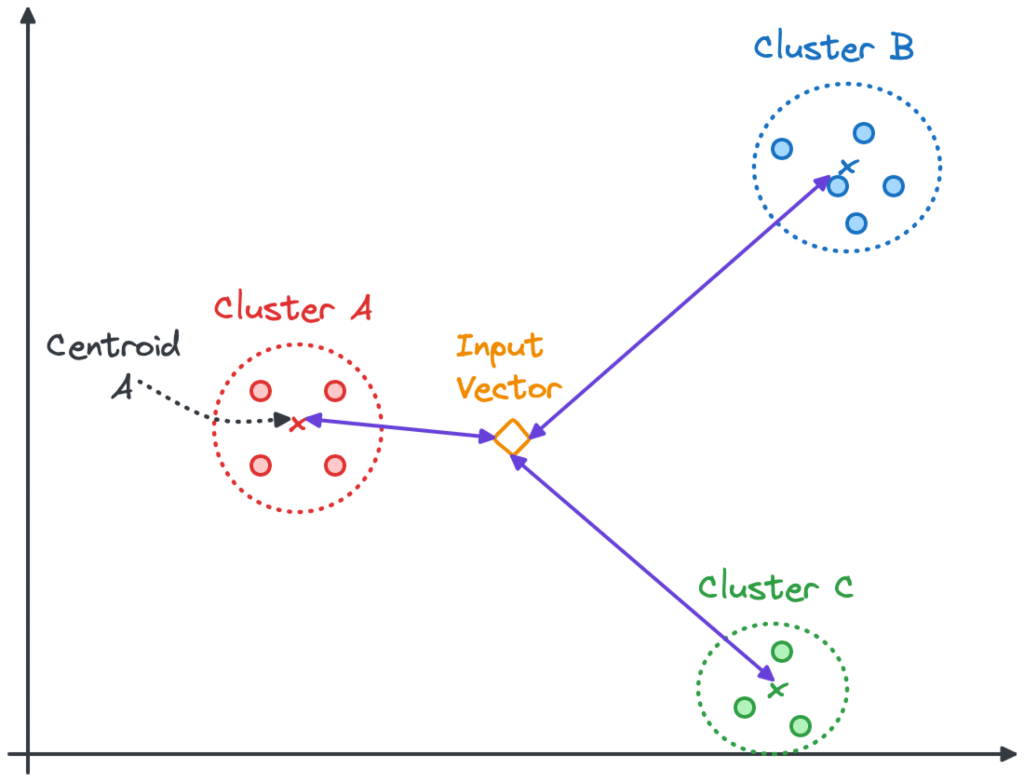
The accuracy and speed of the results depends on the effectiveness of the clustering algorithm. IVFFlat provides two parameters you can tune:

• lists: the maximum number of vectors in a cluster. All clusters have the same maximum number of vectors, but the actual number of vectors in a cluster can vary.
• probes: the number of clusters to examine during the search.

Tuning the IVFFlat lists parameter

A smaller lists parameter creates smaller clusters, with less distance between the vectors and the centroid. However, it increases the number of clusters, making the search less efficient. The image below shows how a change in the lists parameter from 5 to 8 might affect the cluster composition.

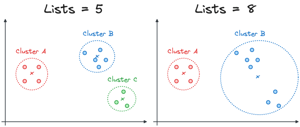
The number of clusters and the distance of the centroid affect the accuracy of the results. In the following visualization we can see how the 4 similar vectors from the input might change in the case when only the closest cluster is inspected. Note that in both cases, one of the closest results is not discovered when the index is used.

How to define the IVFFlat list parameter

The lists parameter is defined during the index creation stage. The pgvector documentation suggests using the following formula for lists as a starting point:

• rows / 1000 for up to 1 million rows
• sqrt(rows) for over 1 million rows

For our testing purposes, let’s create an index with a maximum of 200 vectors in a cluster:

CREATE INDEX idx_articles_ivfflat ON articles USING ivfflat (content_vector vector_l2_ops) WITH (lists = 200);

Creating the index took approximately 15 seconds in my test environment.

Note: Increasing the lists parameter will require more working memory. If your working memory is not enough you could get an error like this:

ERROR:  memory required is 405 MB, maintenance_work_mem is 150 MB.

In such cases, check your server has enough memory and then increase the working memory with a statement like this:

set maintenance_work_mem='500MB';

You can then try entering the index creation statement again.

When you issue a new search query, it will use the index automatically. In some cases, you might need to run:

ANALYZE articles

to force the index to be recognized.

If we issue the same Pineapple Pizza query we used earlier, the results are retrieved much faster (130 ms) but are quite different from the original query.

title    |     similarity
-------------+--------------------
Pizza       | 0.5768115872776731
Pepperoni   |  0.610343554634968
Afelia      | 0.6747670584095107
Ravioli     | 0.6852264524921056
Pot Noodle  | 0.6863169461307689
Coprophagia | 0.6866620332212815
Kalua       | 0.6980457162874122
Andouille   | 0.7013536605444092
Dim sum     | 0.7031395804694845
Doner kebab |  0.704823434748779

(10 rows)

Most of the results from our original results (including Pizza Pizza, Pineapple, and Hawaiian Punch) have disappeared. The new results have less similarity to Pineapple Pizza.

Tuning the IVFFlat probes parameter

Why so much change? It’s because we clustered the vectors in groups of 200 and we analyzed only the cluster with the closest centroid to our input vector, because the probes parameter is 1 by default.

The probes parameter, which can be changed at query time, identifies the number of clusters that PostgreSQL will inspect. In the case of probes=1, only the cluster with the closest centroid to the input vector will be inspected. With probes=N the top N closest clusters will be inspected (see the image below).

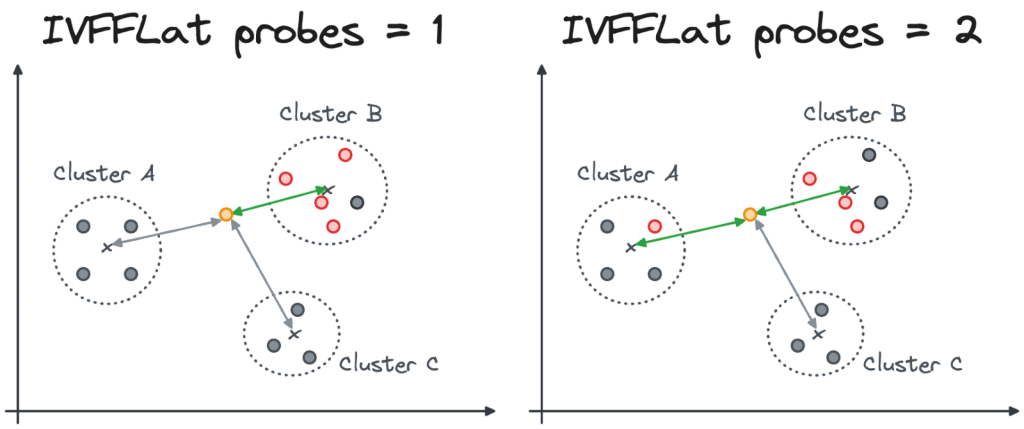
A lower probes parameter speeds up queries at the cost of accuracy. A higher probes number will probably slow down the query, but it will return higher quality results.

How to define the IVFFlat probes parameter

You can change the probes parameter before you run a query. In our example, we can change the probes parameter to 2 with:

SET ivfflat.probes = 2;

If we now issue the same query as before, it displays a result set more aligned with the one retrieved from the non-indexed table.

title    |     similarity
-------------+--------------------
Pizza Pizza | 0.5479716613013446
Pizza       | 0.5768115872776731
Pepperoni   |  0.610343554634968
Pizza Hut   | 0.6337399221217159
Afelia      | 0.6747670584095107
Ravioli     | 0.6852264524921056
Pot Noodle  | 0.6863169461307689
Coprophagia | 0.6866620332212815
Kalua       | 0.6980457162874122
Andouille   | 0.7013536605444092

(10 rows)

This is a good time to talk about performance measurement. When I ran this query, the time taken dropped from 130 ms (probes=1) to 79 ms (probes=2). That means I achieved both higher quality and faster performance, which was unexpected. However, the time scales we’re dealing with are tiny and highly susceptible to effects such as network delay because I was using a cloud service. I recommend you conduct your own speed tests. Results may be more repeatable and more likely to be as expected when working with larger data sets.

Some entries from the original non-indexed results, such as Hawaiian Punch, are not shown. Let’s try increasing the probes parameter to 10:

SET ivfflat.probes = 10;

The query now runs in 208 ms (much faster than the non-indexed 447 ms) and the result set is more aligned with the initial content list.

title      |     similarity
----------------+--------------------
Pizza Pizza    | 0.5479716613013446
Pizza          | 0.5768115872776731
Pepperoni      |  0.610343554634968
Pineapple      | 0.6146698071910883
Pizza Hut      | 0.6337399221217159
Hawaiian Punch | 0.6701219221107402
Pie            |  0.673541906631888
Afelia         | 0.6747670584095107
Pastry         | 0.6821241658509565
Ravioli        | 0.6852264524921056

(10 rows)

The most important takeaway is that increasing the probes parameter increases the accuracy, but also the query time.

Using the pgvector Hierarchical Navigable Small Worlds (HNSW) index

Another approach is the Hierarchical Navigable Small Worlds (HNSW) index. Instead of creating clusters of nodes around centroids, the HNSW index creates layers of increasingly dense linked vectors, as shown in the image below.

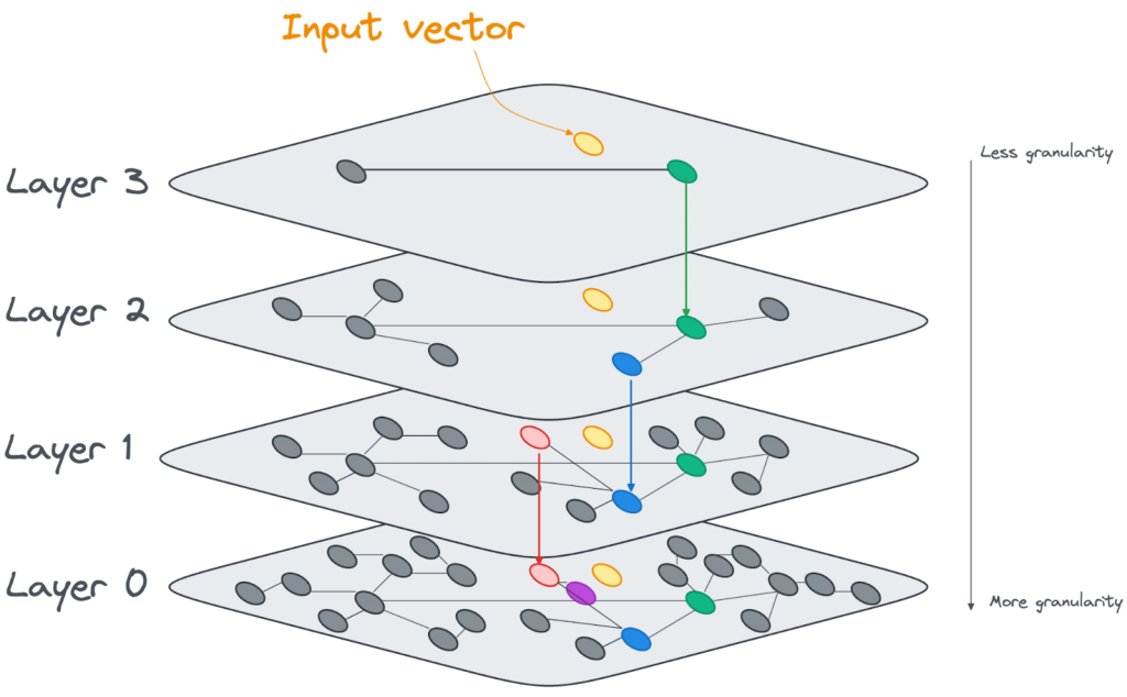
At query time, the search algorithm will start at the top layer and find the nearest vector to the input vector. It then descends through it, and assesses the vectors that are directly linked on the next layer. It keeps descending through the layers and evaluating the distance from the input vector until it generates the closest vector as the result at the bottom layer.

Internally the HNSW indexes are built as linked lists, with an increasing number of nodes added at each layer.

The accuracy and speed of the results depends on how effectively the layers are built. HNSW provides two index creation parameters that we can tune:

• m: the number of connections to nearest neighbors. For every vector on a layer, m defines the number of links to other vectors.
• ef_construction: the number of nearest neighbors to keep in the list while traversing the layer for index creation.

HSNW also provides a parameter tunable at query time, named ef_search. It dictates how many closest neighbors to keep in the working list during the search. The explanation above is simplified by implying there is just one path through the layers. The search can follow multiple paths through the layers, which is why the working list is needed. With a higher ef_search value, more vectors are inspected, which is slower but is likely to deliver better results.

Tuning the HNSW m parameter

A small m parameter will create layers with fewer connections, which are therefore faster to navigate. At the same time, having fewer connections between vectors means that the accuracy could be reduced. There could be a missing link between a node accessed at layerN+1 and the optimal node at layerN as shown in the image below.

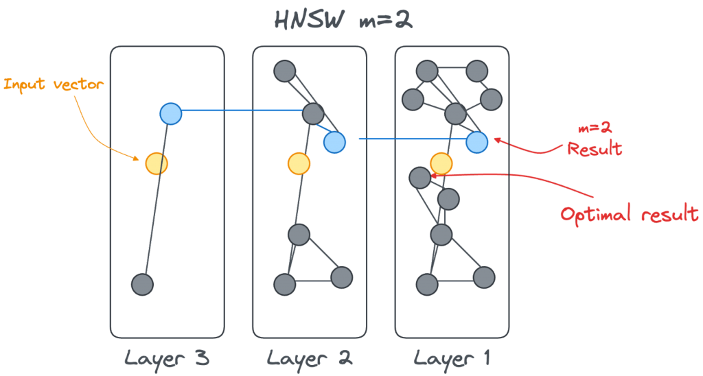
On the other hand, increasing m means the vectors on a level are more connected. There are more chances to find the closest vector, and just not an approximation due to a lack of connections. The improved quality comes at the cost of performance: more connections are available and therefore more connections need to be checked.

Tuning the HNSW ef_construction parameter

The ef_construction parameter defines the size of the closest candidate list used during the index building process. The list contains the closest candidates found so far while traversing the graph. Once the traversal is finished, the list is sorted and only the first m links are kept. See the image below.

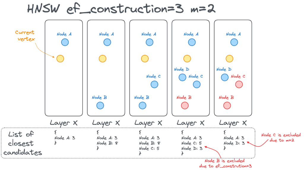
A higher value for ef_construction will likely increase accuracy because more vectors are kept in the working list. But it will take longer to create the index because there are more vectors to evaluate.

How to define the HNSW m and ef_construction parameters

Both the m and ef_construction parameters are defined during index creation. Drop the IVFFlat index created previously with:

DROP INDEX idx_articles_ivfflat;

We can then create the HNSW index with m=10 and ef_construction=40 by entering:

CREATE INDEX idx_articles_hnsw ON articles USING hnsw (content_vector vector_l2_ops) WITH (m = 10, ef_construction = 40);

The HNSW index is slower to build than the IVFFlat index. You can check progress with:

SELECT phase, 
round(100.0 * blocks_done / nullif(blocks_total, 0), 1) AS "%" 
FROM pg_stat_progress_create_index;

Which will show a table like this:

phase              |  %
------------------------------+------
building index: loading tuples | 97.4

(1 row)

This tells us that the index is in the loading tuples stage (the second and final stage) at 97.4%. Our example took 2 min 5 secs to build the HNSW index. That’s quite a lot longer than the 15 seconds of the IVFFlat.

Note: you might hit the following warning:

NOTICE:  hnsw graph no longer fits into maintenance_work_mem after 23852 tuples
DETAIL:  Building will take significantly more time.
HINT:  Increase maintenance_work_mem to speed up builds.

This can be solved by increasing the maintenance_work_mem as discussed for the IVFFlat index.

Time to query! Let’s try our standard query and check the results! The query is now retrieved in only 28 ms and returns exactly the same results as the non-indexed query which took 447.857 ms.

title       |     similarity
----------------+--------------------
Pizza Pizza    | 0.5479716613013446
Pizza          | 0.5768115872776731
Pepperoni      |  0.610343554634968
Pineapple      | 0.6146698071910883
Pizza Hut      | 0.6337399221217159
Te Puke        | 0.6567274128181192
Lanai          | 0.6621790036299536
Hawaiian Punch | 0.6701219221107402
Pie            |  0.673541906631888
Afelia         | 0.6747670584095107

(10 rows)

Tuning the HNSW ef_search parameter

As mentioned earlier, the ef_search parameter dictates the number of closest vectors to keep in the working list during the search. The default value is 40. Let’s check how changing this parameter affects the performance and the accuracy by modifying it to keep only the closest vector in the working list:

SET hnsw.ef_search = 1;

If we now rerun the query, the result set is as shown below:

  title  |     similarity
---------+--------------------
 Pompeii | 0.7384170730225783
(1 row)

There are a couple of things of note:

• The result set contains only 1 row instead of 10: this is because ef_search dictates the number of vectors to keep in the working list, effectively setting a maximum number of results that can be output.
• The retrieved row is not the one with highest similarity: since we are only keeping the closest vector during our descent through the layers, we found a local optimum and not the overall optimum result. The new result is both new and not closely related to the query.

Let’s now increase ef_search to 5:

SET hnsw.ef_search = 5;

Again, the result set seems stuck in a local optimum, far from the expected results:

title          |     similarity
-------------------------+--------------------
Afelia                  | 0.6747670584095107
Pianosa                 | 0.6796609500654267
Estádio Palestra Itália |  0.711623227925174
Giannutri               | 0.7129644486337057
Gorgona, Italy          |  0.714280954413222

(5 rows)

Raising the ef_search parameter to 20 gives us a result set closer to the expected results:

title      |     similarity
----------------+--------------------
Pizza Pizza    | 0.5479716613013446
Pizza          | 0.5768115872776731
Pepperoni      |  0.610343554634968
Pineapple      | 0.6146698071910883
Pizza Hut      | 0.6337399221217159
Te Puke        | 0.6567274128181192
Lanai          | 0.6621790036299536
Hawaiian Punch | 0.6701219221107402
Pie            |  0.673541906631888
Afelia         | 0.6747670584095107

(10 rows)

HNSW vs IVFFlat: Which to use?

The tests we’ve done and their results provide a nice overview of the two indexing options we have. The next question is: which one should I choose?

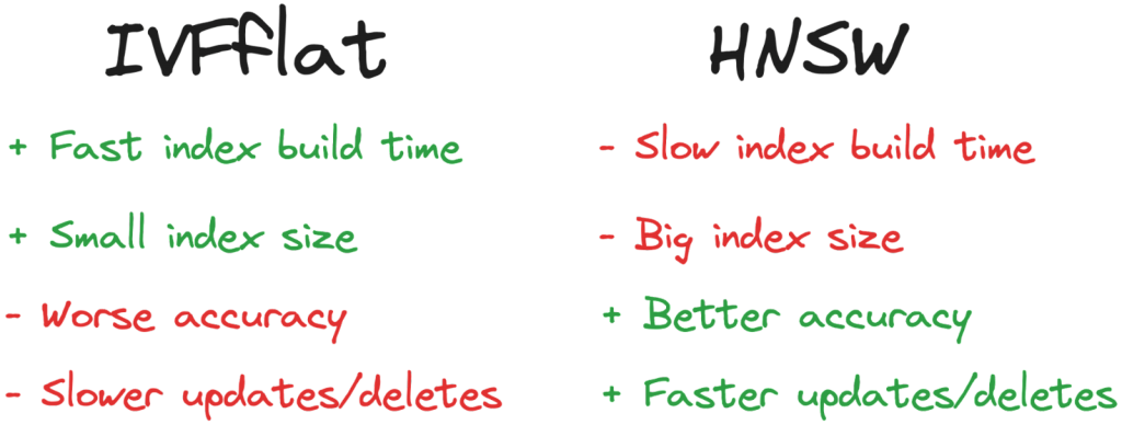
The reply is, as always, it depends: IVFFlat indexes are usually faster to build and smaller in size, but, on the other hand, are slower to use and less accurate. If your main optimization objective is to speed up the index creation phase or to keep the index size to a minimum, then IVFFlat is your best option. On the oth, though, you want to maximize both accuracy and query speed, then choose HNSW.

If you are carrying out a lot of updates and deletes on the database, HNSW is the better option. The IVFFlat clustering mechanism would need to be rebuilt, but HNSW can remove vectors from the internal linked list easily, taking less time.

Additional techniques to speed up vector indexes

The above techniques assume we want to create an index across the entire data set. However, we can use standard PostgreSQL performance improvements to further speed up certain types of queries.

Partial indexes

For example, if we only care about indexing a particular subset of the data, we can apply a WHERE condition during the index creation process, like this:

CREATE INDEX idx_articles_hnsw ON articles 
    USING hnsw (content_vector vector_l2_ops) 
    WITH (m = 10, ef_construction = 40) WHERE id < 4000;

This will index only the rows having an id less than 4000, resulting in a smaller and faster index for queries that are looking within this segment of data.

If we add WHERE id between 1 and 1000 to our original query, using EXPLAIN will show the idx_articles_hnsw index is being used:

-----------------------------------------------------------------------------------------------
QUERY PLAN
-----------------------------------------------------------------------------------------------
 Limit  (cost=41.30..67.74 rows=10 width=21)
   ->  Index Scan using idx_articles_hnsw on articles  (cost=41.30..916.62 rows=331 width=21)
         Order By: (content_vector <-> '[....]'::vector(1536))
         Filter: ((id >= 1) AND (id <= 1000))
(4 rows)

(END)

Table partitioning

If we want to index the whole data set, but we are happy to create different vector indexes based on categorizing the data, then we can use partitioned tables with dedicated indexes for each partition.

In our Wikipedia example, we can create a table that partitions the data based on the hashing of the title column with:

CREATE TABLE IF NOT EXISTS articles_partitioned (
    id INTEGER NOT NULL,
    url TEXT,
    title TEXT,
    content TEXT,
    title_vector vector(1536),
    content_vector vector(1536),
    vector_id INTEGER
)
PARTITION BY hash(id);
CREATE TABLE articles_partitioned_p_hash_p1 partition of articles_partitioned for values with (modulus 10, remainder 0);
CREATE TABLE articles_partitioned_p_hash_p2 partition of articles_partitioned for values with (modulus 10, remainder 1);
CREATE TABLE articles_partitioned_p_hash_p3 partition of articles_partitioned for values with (modulus 10, remainder 2);
CREATE TABLE articles_partitioned_p_hash_p4 partition of articles_partitioned for values with (modulus 10, remainder 3);
CREATE TABLE articles_partitioned_p_hash_p5 partition of articles_partitioned for values with (modulus 10, remainder 4);
CREATE TABLE articles_partitioned_p_hash_p6 partition of articles_partitioned for values with (modulus 10, remainder 5);
CREATE TABLE articles_partitioned_p_hash_p7 partition of articles_partitioned for values with (modulus 10, remainder 6);
CREATE TABLE articles_partitioned_p_hash_p8 partition of articles_partitioned for values with (modulus 10, remainder 7);
CREATE TABLE articles_partitioned_p_hash_p9 partition of articles_partitioned for values with (modulus 10, remainder 8);
CREATE TABLE articles_partitioned_p_hash_p10 partition of articles_partitioned for values with (modulus 10, remainder 9);

We can insert the data into the articles_partitioned table with:

INSERT INTO articles_partitioned SELECT * FROM articles;

We can now create an index like this:

CREATE INDEX idx_articlespartitioned_hnsw ON articles_partitioned 
    USING hnsw (content_vector vector_l2_ops) 
    WITH (m = 10, ef_construction = 40);

The index is created pretty fast, but the results are not as accurate as before:

title    |     similarity
-------------+--------------------
Pizza Pizza | 0.5479716613013446
Pepperoni   |  0.610343554634968
Pineapple   | 0.6146698071910883
Pizza Hut   | 0.6337399221217159
Te Puke     | 0.6567274128181192
Pie         |  0.673541906631888
Afelia      | 0.6747670584095107
1518        | 0.6799215593395357
Pastry      | 0.6821241658509565
Ravioli     | 0.6852264524921056

(10 rows)

The accuracy is lower because PostgreSQL creates an index per partition. From the similarity search point of view, it creates layers or clusters based only on data contained in a single partition (see the image below).

This approach is good if we know our search will always hit data in just one partition. For example, if we partition the table based on products, searching within a particular product category will work well. If a search is done across partitions, for example looking for items with similar designs across different product categories, there may be suboptimal results. In our pizza example, we partitioned by hashing the id and the query spanned all the partitions, so the accuracy was lower.

Hybrid search with index combination

You might be wondering whether it’s possible to combine an index with a hybrid search, to speed up combined searches of vectors and standard data columns. Unfortunately, it isn’t yet.

Check our article to learn what is the best PostgreSQL index based on your query

You might think we could index the vector and standard data columns separately and that PostgreSQL could combine the results of the indexes.

For example, let’s consider the following query (the vector data is hidden in the SQL):

select title, 
content_vector <-> vt similarity
from articles
where id = 1000
order by content_vector <-> [........]
limit 10;

Our data set is somewhat limited, so for demonstration purposes we’ll search by ID as well as the article content, even though the ID is just a sequential number. Let’s create an index on the articles column id:

create index idx_id on articles(id);

Our hope is that PostgreSQL will use both indexes to retrieve the results without accessing the table. However, PostgreSQL only uses the index on the content_vector column to find the nearest vectors and then filters the result using the id column, as shown by EXPLAIN:

Limit  (cost=61.45..64.54 rows=10 width=21)
   ->  Index Scan using idx_articles_hnsw on articles  (cost=61.45..7673.61 rows=24666 width=21)
         Order By: (content_vector <-> '[...]'::vector(1536))
         Filter: (id > 1000)
(4 rows)

While this returns the right results, it doesn’t give us the speed benefit of using an index on the id column.

Unfortunately, you can’t create multi-column indexes that mix vector and standard data. Let’s try, for example, to add multiple columns to an hnsw (or ivfflat index) like this:

CREATE INDEX idx_articles_hnsw ON articles 
    USING hnsw (content_vector vector_l2_ops, id) WITH (m = 10, ef_construction = 40)

We get the following error:

ERROR:  access method "hnsw" does not support multicolumn indexes

We could try to do this with the INCLUDE option like this:

CREATE INDEX idx_articles_hnsw ON articles 
    USING hnsw (content_vector vector_l2_ops) INCLUDE (id) WITH (m = 10, ef_construction = 40)

But this results in a similar error:

ERROR:  access method "hnsw" does not support included columns

Since hybrid search is becoming more popular, we expect methods like this to be supported in the future. Looking at the pgvector GitHub repository, there’s an active discussion about combining HNSW and filtering in a unique index. Moreover, a branch was recently created as a first attempt to implement the HQANN search. This should allow scalar and vector types to be mixed in the same index using a modified distance function. It’s worth keeping an eye on both of these developments because hybrid searches are a common requirement.

Please note that hybrid queries are still possible in PostgreSQL, they will only partially use one of the index available.

Indexes to avoid full vector element comparison

The indexes we’ve explored allowed us to avoid scanning the full table, but this is only one of the optimization options when dealing with vectors. The other is to reduce the amount of work by shortening the vector size: instead of comparing 1536 elements per array, why don’t we compare only a subset (for example, 256) of them?

In the past, this wouldn’t work because models were trained with a specific embedding length in mind and gave each element equal weight. Skipping some embeddings would mean arbitrarily discarding useful information. But more recent models, such as OpenAI text-embedding-3-large, provide a native way to shorten embeddings, without losing too much accuracy. In technical terms, this is called Matryoshka representation learning.

When using models which have the embeddings shortening feature, we can work with a subset of the elements, usually taking the first chunk in predefined sizes (for example 256, 512 or 1024.

Shortening the vector size in PostgreSQL

How do we shorten the vector size? You might think you could use subscripting:

SELECT content_vector[1:256] FROM articles;

Unfortunately this doesn’t work, giving you the following error:

ERROR:  cannot subscript type vector because it does not support subscripting.

You could try to cast the vector as an 256-item array of float:

select content_vector::FLOAT[256] from articles;

But this also fails:

ERROR:  cannot cast type vector to double precision[].

What we can do is cast the vector as text and then as an array like this:

select translate(((translate(content_vector::text, '[]','{}')::FLOAT[])[0:256]::text), '{}','[]')::vector(256) 
from articles 
limit 1;

In the above we:

• convert the content_vector to text
• substitute the [ and ] with { and }
• cast the result to a FLOAT array
• take the first 256 entries from the resulting array via subscripting ([0:256])
• substitute the { and } with [ and ]
• Convert back to text
• cast the result back to vector

Indexing a shortened vector in PostgreSQL

How can we speed up the search query? We could create an index on the entire expression for creating the shortened vectors like this (paste the first 256 elements of the query into the second line):

with data as (
    select '[first 256 elements of the OpenAI vector]'::VECTOR(256) as vt
)
select title, 
    translate(((translate(content_vector::text, '[]','{}')::FLOAT[])[0:256]::text), '{}','[]')::vector(256) <-> vt similarity
from articles_partitioned join data on 1=1
order by translate(((translate(content_vector::text, '[]','{}')::FLOAT[])[0:256]::text), '{}','[]')::vector(256) <-> vt
limit 10;

This code runs, without indexes, in 30 sec and is creating the 256 element version of the embeddings.

We could try to create the index with:

CREATE INDEX idx_articles256_hnsw ON articles_partitioned 
    USING hnsw ((translate(((translate(content_vector::text, '[]','{}')::FLOAT[])[0:256]::text), '{}','[]')::vector(256)) vector_l2_ops) 
    WITH (m = 10, ef_construction = 40);

But that fails with the following error:

ERROR:  functions in index expression must be marked IMMUTABLE.

What’s more, indexes over functions are not a great technique because they force users to use the same complex syntax to query them.

An alternative is to create an additional column in the articles table to store the 256 element vectors:

ALTER TABLE articles ADD COLUMN content_vector_reduced VECTOR(256);

We can populate it like this:

UPDATE articles SET content_vector_reduced=translate(((translate(content_vector::text, '[]','{}')::FLOAT[])[0:256]::text), '{}','[]')::vector(256);

And create the index on the 256 element version with:

CREATE INDEX idx_articles256_hnsw ON articles 
    USING hnsw (content_vector_reduced vector_l2_ops) 
    WITH (m = 10, ef_construction = 40);

Creating this index is way faster (15 sec).

We can now try this query, limiting the input vector to the first 256 elements of the original array:

with data as (
    select '[
    0.02338707074522972, -0.017537152394652367, 0.014360039494931698, -0.025202563032507896, -0.017234569415450096, 0.0018643466755747795, -0.013893559575080872, -0.009581765159964561, 0.006732450798153877, -0.03714194521307945, 0.021848944947123528, 0.008800094947218895, -0.012323915027081966, 0.005071401130408049, -0.0010046670213341713, 0.008768576197326183, 0.03086336888372898, -0.010867739096283913, -0.001483755186200142, -0.006631589960306883, 0.00044835725566372275, -0.01773887313902378, 0.01492738164961338, -0.01236173789948225, 0.022340642288327217, 0.009815005585551262, 0.008579461835324764, -0.00020428228890523314, 0.011605282314121723, 0.014309609308838844, 0.05285099893808365, -0.0039430223405361176, -0.012985813431441784, -0.01689416542649269, -0.02065122500061989, 0.0007375437417067587, -0.003873680718243122, -0.010886650532484055, 0.001689416472800076, -0.022769300267100334, 0.01762540452182293, -0.03451956808567047, -0.009644802659749985, -0.023160135373473167, -0.042336273938417435, 0.0012576066656038165, -0.002456903224810958, -0.01002933457493782, -0.0002019183593802154, -0.01362880039960146, 0.018482720479369164, 0.009733055718243122, -0.028140131384134293, -0.005036730319261551, 0.005433869548141956, 0.010357131250202656, -0.0082012340426445, -0.023424893617630005, -0.00740065285935998, -0.01778930239379406, 0.01135313045233488, 0.0030967381317168474, -0.03149374946951866, 0.003227541921660304, -0.0014018059009686112, 0.005799489561468363, 0.003656199900433421, -0.011605282314121723, 0.021647224202752113, -0.008012120611965656, 0.021382465958595276, 0.007583462633192539, 0.01825578324496746, -0.02455957606434822, 0.013111889362335205, 0.006612678524106741, -0.01002933457493782, -0.013843129388988018, 0.0011441383976489305, 0.009436777792870998, 0.026501145213842392, -0.012424775399267673, 0.0019179289229214191, 0.038327060639858246, 0.017511935904622078, 0.0007111466256901622, -0.0398399718105793, 0.014902166090905666, 0.01705806329846382, -0.0058120968751609325, -0.01645289920270443, 0.005802641157060862, -0.0021842641290277243, 0.013200142420828342, -0.038629643619060516, 0.012626497074961662, -0.011674623936414719, 0.025063879787921906, 0.004006060305982828, -0.02570686675608158, -0.0014152014628052711, 0.01905006170272827, -0.014082673005759716, -0.02687937207520008, 0.002307188231498003, -0.007684323471039534, -0.0012316035572439432, -0.023550970479846, 0.023122312501072884, 0.0026712322141975164, -0.011838522739708424, 0.03119116649031639, 0.010023030452430248, -0.022907983511686325, 0.002924959873780608, 0.004500907845795155, 0.015116495080292225, 0.007148500997573137, -0.024143526330590248, -0.04362224414944649, 0.028316637501120567, 0.0036971743684262037, 0.027333244681358337, -0.00706024793908, 0.02720716968178749, 0.0025388526264578104, 0.001517638098448515, -0.021458109840750694, 0.004188870079815388, -0.0099032586440444, 0.027434106916189194, 0.00335992150940001, 0.013729660771787167, -0.005878286901861429, -0.0066757164895534515, 0.005052489694207907, -0.011208144016563892, -0.017511935904622078, -0.02303405851125717, -0.04329444840550423, 0.016087278723716736, 0.03217455744743347, -0.020260389894247055, 0.02179851569235325, -0.02310970425605774, 0.01286604069173336, 0.014196141622960567, 0.008674019016325474, -0.007785184308886528, -0.018268391489982605, 0.02343750186264515, 0.00034887553192675114, 0.0004243240400683135, 0.009991511702537537, 0.014435685239732265, 0.0001373044797219336, -0.028417497873306274, 0.011056852526962757, 0.005695476662367582, -0.009323309175670147, 0.010016726329922676, -0.016490722075104713, -0.010924472473561764, -0.008692930452525616, 0.012815610505640507, 0.03946174308657646, 0.004904350731521845, 0.023513147607445717, -0.0021291060838848352, -0.005043034441769123, -0.0021763844415545464, 0.04074771702289581, -0.042714498937129974, 0.025719475001096725, -0.007028728723526001, 0.007659108377993107, -0.018596189096570015, -0.003369377227500081, 0.01211589016020298, 0.011662016622722149, -0.005188021343201399, -0.00453557912260294, 0.013414471410214901, 0.032729290425777435, -0.01222305465489626, -0.03595683351159096, -0.00804994348436594, -0.027333244681358337, -0.007898651994764805, -0.005610375665128231, 0.013326218351721764, 0.028467928990721703, 0.01912570744752884, 0.0004979996010661125, -0.6854491829872131, -0.014700444415211678, 0.01694459468126297, -0.04112594574689865, 0.022857552394270897, 0.042058903723955154, 0.005216388497501612, -0.010672321543097496, -0.0071232859045267105, -0.022605400532484055, -0.003879984375089407, 0.017776696011424065, 0.038377489894628525, -0.0006792336935177445, -0.02174808457493782, -0.023160135373473167, 0.018217960372567177, -0.013225357048213482, -0.016162924468517303, 0.020840339362621307, -0.0008691354305483401, 0.0037728198803961277, 0.01689416542649269, 0.00024269602727144957, 0.040016476064920425, 0.0029958775267004967, 0.018570972606539726, -0.015683837234973907, -0.004273971542716026, 0.013691837899386883, -0.02469825930893421, 0.008888348005712032, 0.005310945212841034, -0.00878748670220375, 0.047707103192806244, 0.009272878989577293, -0.03192240744829178, 0.01286604069173336, 0.00370032642967999, 0.03729323670268059, -0.010212143883109093, -0.018709657713770866, 0.02627420797944069, 0.0015113343251869082, -0.024710867553949356, -0.00931700598448515, 0.016818519681692123, -0.0068270075134932995, 0.014813913032412529, -0.007778880186378956, 0.02179851569235325, 0.0021338339429348707, 0.0198065172880888, 0.021861553192138672, 0.0033473139628767967, -0.00144593243021518, 0.03991561755537987, 0.00053385243518278, -0.0048034898936748505, -0.008409259840846062, -0.0037034782581031322, 0.008276879787445068]'::VECTOR(256) as vt
)
select title, content_vector_reduced <-> vt similarity
from articles join data on 1=1
order by content_vector_reduced <-> vt
limit 10;

The result set comes back in 24 ms with the top results in line with the original non-indexed query, as shown below. The similarity figures are much lower than our original search because the similarity calculation uses fewer elements.

     title      |      similarity
----------------+---------------------

 Pizza          | 0.22997463729171275
 Pizza Pizza    | 0.23568754629581293
 Pepperoni      | 0.24703888071231495
 Pineapple      | 0.25392144964646235
 Pie            | 0.27119107491923206
 Pizza Hut      | 0.27250517892728304
 The Republic   |  0.2727779881779113
 Grape tomato   |  0.2736757330550383
 English muffin | 0.27480416043684464
 Pastry         |  0.2783681192665386


(10 rows)

Conclusion

Pgvector is a very powerful backend for your AI applications. The ability to store embeddings and calculate vector similarity, together with the huge set of PostgreSQL SQL features, enables users to mix standard queries and AI-driven searches to provide better results.

Indexing can speed up performance when the amount of data or the size of the embeddings are a challenge. The IVFFlat and HNSW indexes allow you to cluster similar embeddings or layer the vector search queries. Shortening the vector size speeds up performance at the cost of accuracy.

In the vector space there’s no free food: performance and accuracy are a tradeoff when using indexes. Analyzing the indexing parameters and how they influence the query behavior can help you to define the sweet spot between the query speed and the accuracy of the results.

For more SQL tuning tips, check out our SQL optimization guide!